So to recap, ray tracing is a computational model utilised in attempting to render photo-realistic 3D images.
You see the world around you by a process whereby the sun emits rays of light (a great read here: it emits around 1045 every second!), most of which go out in to space never to be seen again. A tiny fraction of them land upon the earth. Some of those photons bounce off the sky and get a bit of a blueish tint (c.f. science – why is the sky blue). Some of the photons bounce off (my terminology!) objects around you and turn the colour of that object. Some of those bounce off other objects (stop me if my science lessons is getting either too complicated, or too correct!), come through your windows. And so on.
And a tiny, tiny, tiny fraction of the sun’s original photons, having done all that, pass in to your eyeball, get absorbed and turned in to electrical signals, which are then all joined up in your brain into the stuff you can see.
(Move over Jim Al-Khalili!)
Ray tracing assumes that trying to mathematically compute all of the above would be a bit dumb and so instead calculates all of the above above in reverse. As if your eye is sending out little feeler rays out in to the world to see what colour the object they reach is, and how much light might then have reached that place.
Moreover, since the image is going to be ultimately rendered on a computer screen or similar, it tends to work in a pixellated way. Effectively sending out a detecting-ray asking “what’s out there?” out through every pixel on the screen into the world-at-large.
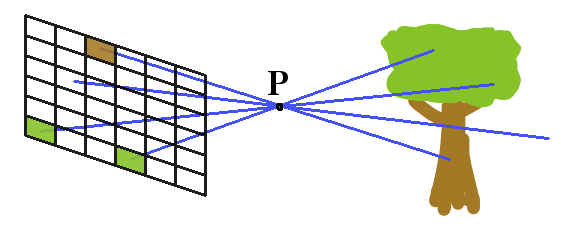
The simple model works in one of two ways. Either directly modelling how a pinhole camera works. Sending out a detection-ray through a common point in space (a.k.a. the theoretical pinhole), and seeing a picture of the world upside-down:
Or by kind of working out where your viewpoint is in relation to the rendering screen (a.k.a. viewframe) and doing the maths that way round:
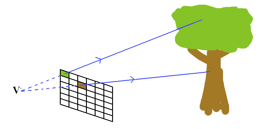
It’s a pretty arbitrary decision, and as it happens I’ve gone with the second choice. Ironically enough, although I’m counting my top-left pixel as pixel #1, and working right and down that round, the drawing function I’m currently using thinks of its origin as the bottom left corner of the screen, so my image is both upside-down AND back to front by that measure. It’s all just maths. Doesn’t matter…
At some point I hope to take the model a little bit further and add in some maths to mimic the optics of a proper lensed camera. It gets much more exciting then, with depth of field, focus and all sorts of exciting stuff like that. But again it’s all just maths, and that stuff is totally modular, so I’m ignoring that for the time being…
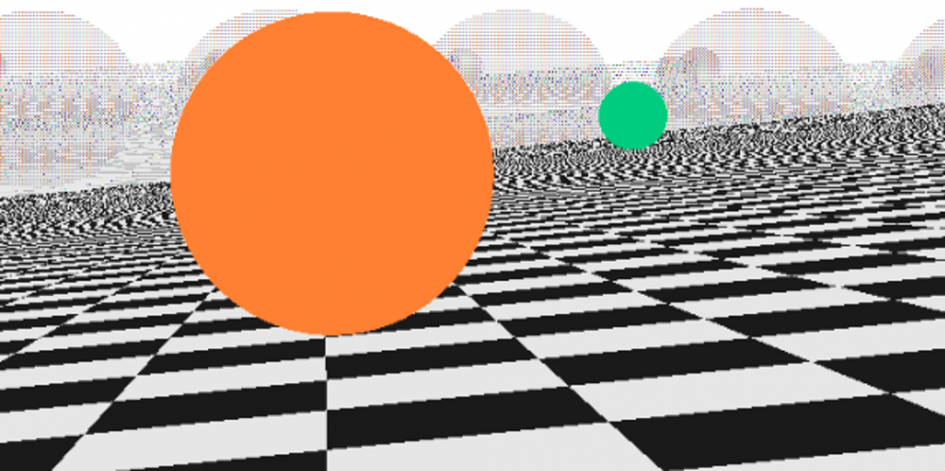
Here’s where I’ve got to so far
I’m pretty darned chuffed with this, even though it’s still early days.
(Note, the headline image at the very top of this page, which I’ve entitled “Death Star Anomaly” is an artefact of either some slight oddness in the rendering package I’m calling, or possibly some sort of memory leakage in the R executable itself, or just a disturbance in the Force. Not sure. It’s not my code, put it that way.)
But I digress, the main point of this exercise is to learn my way around R, so let’s look at that side of things:
Looping in R
So, for the sake of argument, let’s say I’m trying to render a 300×200 pixel image.
The iterative programmer demon on my left shoulder instinctively wants to write some code with begins something like:
for (i in 1:(300*200)) {
  etc...
and then ultimately write the resulting colour of each pixel back to a 60,000 long vector or something like that.
It seems to do a job, but the set-operation angel over my other shoulder can’t help me thinking it’s not the R way of doing things. It’s just not atomic enough.
So here are some thoughts on the matter:
- The apply() family of functions family can achieve the latter approach. I definitely need to get more familiar/comfortable with these!
- But to be honest, from early performance testing to compare the two approaches seems to suggest that there’s absolutely no overhead with the for..loop approach.
- Must investigate R’s parallel processing capabilities. We have RevoScaleR in work as part of a SQL Server 2016 build. That can achieve parallel, although I notice that the copy I have access to is on a single-core server. Hmmm…
Where I have been able to achieve some significant improvement (let’s say 1000s of times faster!) is by not dynamically extending my results vector. Back to my for..loop approach, I was coding something similar to:
pixel.array <- character(0)
for (i in 1:(image.width * image.height)) {
  pixel.array(i) <- ray.colour(viewframe[i]$origin, viewframe[i]$direction)
}
and letting R dynamically extend the length of the pixel.array result vector as it went.
It turned out that’s a slightly naive approach. It seemed to work OK for my 200×200 pixel test run. Took a few seconds to run (need to make some performance tweaks!), so I naturally assumed it would take exactly 25 times longer to process a 1000×1000 pixel image.
Did it bugger! I sat there for ages and ages while my code churned and churned. It seems that allowing R to dynamically extend vectors one at a time really doesn’t work over large vectors like that!
One that can actually be solved by simply filling the length of the vector after initialising it:
pixel.array <- character(0)
#initialise it to NAs
pixel.array[image.width * image.height] <- NA
for ( etc...
A quick demo to prove the point. It’s merely (obviously pointlessly) looping to fill the vector with zero values, in reality it’d call a function for each element. You can run it yourself if you have the patience:
n <- 100000

#Version 1 : simple and efficient
 system.time( x <- rep(0, n))

#Version 2 : just don’t do this!
 system.time( { x <- numeric(0); for (i in 1:n) x[i] <- 0 } )

#Version 3 : same thing, but initialing the vector!
 system.time( { x <- numeric(0); x[n] <- NA; for (i in 1:n) x[i] <- 0 } )
I’d originally coded the demo to build a million element vector, but had to kill Version 2 after 20 minutes or so, as my laptop was getting a little warm!
The code above gave the following timings for me:
- Version 1 : 0.001 seconds
- Version 2 : 41.043 seconds
- Version 3 : 0.156 seconds
And perhaps if nothing else this demonstrates that while for..loop code can perform relatively OK, it needs to be treated with care!
Data structures in R
I love this. It’s so easy!
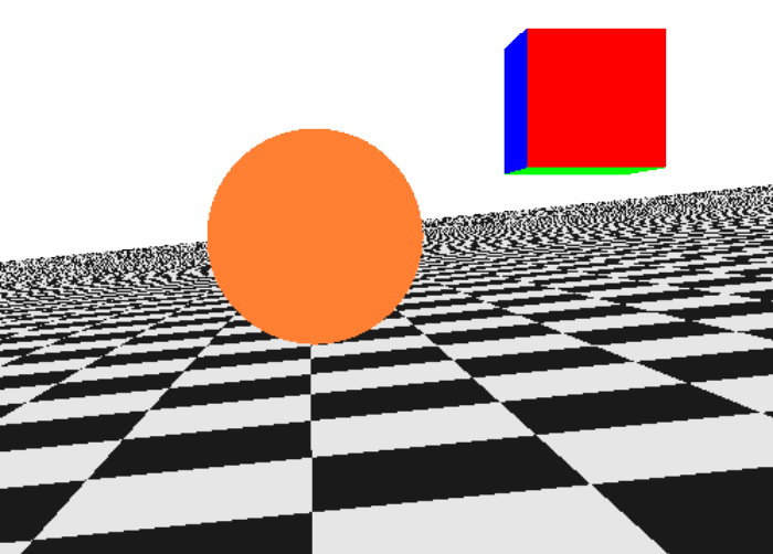
Here’s my world rendered another way. I wrote the code for this wire-frame version mainly because it’s quite fiddly to build up a “world” out of objects placed in 3D space made out of (x,y,z) coordinates, and be able to visualise where everything sits in relation to each other is pretty hard using nothing but ones imagination. So a quick bit of line-rendering code is quite useful to have during this process.
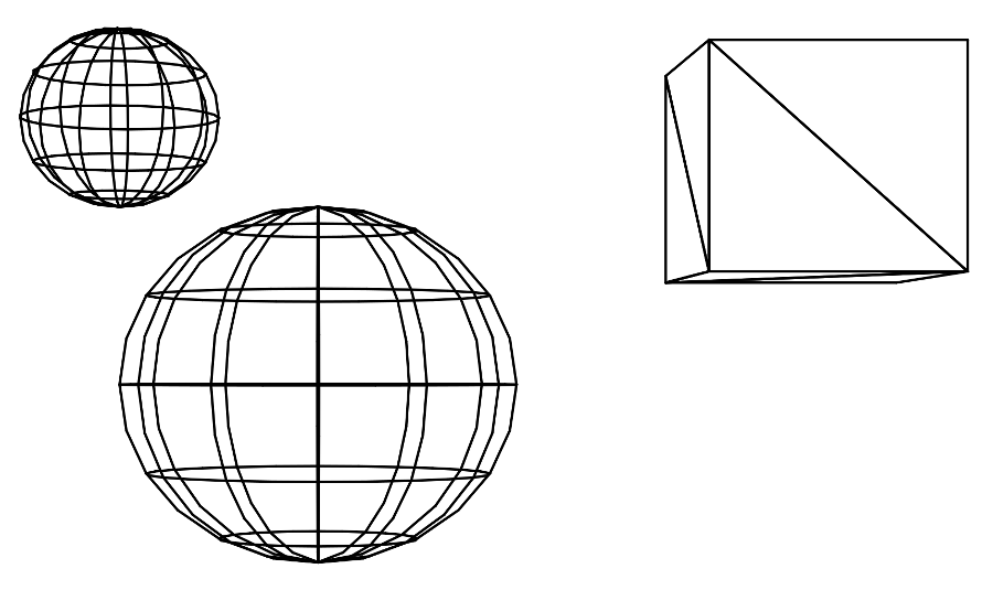
It’s a good way to visualise how my world is currently built. Everything in it is one of:
- A sphere
- A plane (currently in infinite directions)
- A triangle
The cube you see is actually just made of triangles. Actually it’s not even a cube at the moment… I cheated slightly at this stage in the proceedings, since my fledgling ray tracing code can currently only see 3 sides of the cube, since it’s not tracing any secondary rays, shadow effects, lighting etc..
Each one of these objects can be geometrically defined simply by a set of numbers, but exactly what numbers differs for each type:
A sphere is a single point (all points are simply a vector of x, y and z coordinates) and a radius (positive value).
A plane can be defined by the position of one point on the plane, and a trio of numbers defining a directional “normal” vector orthogonal to the plane.
A triangle can be defined by the coordinates of its 3 vertices V1, V2, and V3 – the only mathematical stipulation being that they are 3 different points and not 3 points along a common line in space.
And lists are the perfect storage for this information! In code, something like:
sphere1 <- list(loc=c(x1,y1,z1), radius=r)
plane1 <- list(point=c(x2,y2,z2),normal=c(x3,y3,z3))
triangle1 <- list(v1=c(x4,y4,z4), v2=c(x5,y5,z5), v3=c(x6,y6,z6))
which rather tidily can then be combined as:
world <- list(sphere1, plane1, triangle1)
In version 2 of this, we can build upon this simple list() approach by implementing spacial indexing by adding a slightly deeper hierarchy of objects and virtual bounding volumes, in order to make the code more efficient, but that can wait for now.
Now we have our world object, in order want to trace the path of a given ray we can simply cycle through the list of objects and ask if the ray intersects with each object in turn, until we find the closest intersection point, and therefore the object (and further surface properties thereof), upon which it lies.
And given all of this, the very obvious approach is…
Object oriented
Which again, is something that’s so beautifully simple in R!
Remember when we defined our primitive objects earlier, we could quite easily have also assigned a class to each with a simple extra statement
sphere1 <- list(loc=c(x1,y1,z1), radius=r)
class(sphere1) <- append(class(sphere1,"sphere"))
And having similarly assigned a class to each primitive object in this way, we can then build a generic intersect method function with:
intersect <- function(ray.origin,ray.direction,obj) {
  UseMethod("intersect", obj)
}
Plus an intersect function for each object, which in its current form simply returns a numerical value giving the distance along the ray which the ray and object intersect (or NA otherwise). Here’s the code for the ray/plane intersection, as per the maths on wikipedia:
intersect.plane <-function(ray.origin,ray.direction,plane) {
  t <- sum((plane$point - ray.origin) * plane$normal) /
       sum( ray.direction * plane$normal)
  if (t > 0)
    return (t)
  else
   return (NA)
}
And having written similar functions for each primitive object, our code can simply call the generic intersect function against any given object and let R work out how to do that:
intersect.distance <- intersect(ray.origin, ray.direction, any.given.object)
That’s all for now!
I’ll put the code up on github when I get the chance!
Leave a Reply